Simple SSIS: Date Formats

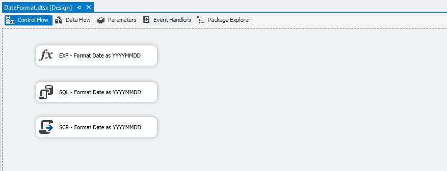
One feature that I would like to see added to SSIS is the ability to format a date string with a specified format. I have been tasked many times with outputting file names or folders with a specific date format, such as YYYYMMDD, and found myself writing custom functionality to accomplish this task. This is not difficult in T-SQL, but in SSIS it’s not all that easy. In this blog post I am going to show a few ways that we can format a date string into a specific format. I will show how to use an Expression task, SQL task, and a Script task.

DateFormat_SSISPackage

Expression Task

EXP – Format Date as YYYMMDD
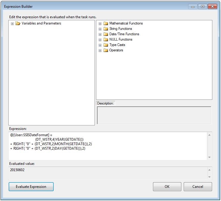
The expression task is a new features with 2012 which allows us to store the result of an expression in a variable. Basically we create an expression using the Expression Builder window and store the result into a SSIS variable. In the windows below you can see an example of the expression being set to the SSISDateFormat variable.

@[User::SSISDateFormat] =  
               (DT_WSTR,4)YEAR(GETDATE())  
+ RIGHT ( "0" + (DT_WSTR,2)MONTH(GETDATE()),2) 
+ RIGHT ( "0" + (DT_WSTR,2)DAY(GETDATE()),2)

DateFormat_ExpressionBuilder


SQL Task

SQL – Format Date as YYYYMMDD
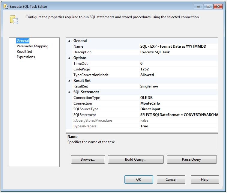
The SQL Task is a commonly used task in SSIS. This task allows us to execute queries against a data source and return a full result set, a single row, or nothing at all. We also have the opportunity to pass variables into the query as well. However, for this example we will not pass anything in, and only return back a single row. Using T-SQL’s CONVERT function it’s very easy to format a date string. We will use this CONVERT function and return the single row and store the results into a SSIS Variable. The SQL syntax that we will use is:

SELECT SQLDateFormat = CONVERT(NVARCHAR(8),GETDATE(),112);

Here is a link to additional formats for the CONVERT function. https://technet.microsoft.com/en-us/library/ms187928.aspx

DateFormat_SQLTask


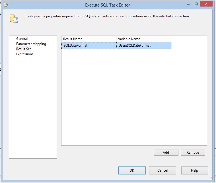
After the SQL Task executes the result will be stored in the SQLDateFormat SSIS variable, which is configured in the window below.

DateFormat_SQLTaskVariables


Script Task

SCR – Format Date YYYYMMDD
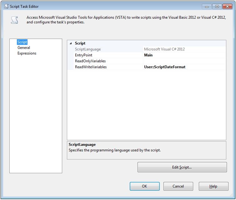
The script task is one of my favorite tasks, mainly because all of the additional functionality that I have access too, but it also gives me an opportunity to play with C#.net code. By passing the SSIS variable ScriptDateFormat into the ReadWriteVariables box, we can access that variable through code. In programming languages like C#.net it’s very easy to format a date string. There is a ToString() method that provides many date formats by using specific characters. When we click on the Edit Script button the Visual Studio for Apps design time environment appears. We can access the ScriptDateFormat variable through the Dts.Variables array and save string values to it. The result of C#.net DateTime.Now.ToString(“yyyyMMdd”) method call will give us a formatted date, this formatted date we can save to our Dts.Variables array. To get a date in T-SQL we use the GETDATE and in C#.net we use DateTime.Now. So the entire line of code would look like this.

Dts.Variables["ScriptDateFormat"].Value = DateTime.Now.ToString("yyyyMMdd");

Here is a link to MSDN page that has the format specifiers.
https://msdn.microsoft.com/en-us/library/8kb3ddd4.aspx

DateFormat_ScriptTask


Summary

So which is the best way? I personally prefer the Script task, mainly because it’s clean and simple. The Expression Task is a complicated expression, and the SQL Task involves an unnecessary round trip to the server to get a formatted date string. With that said, all three options work and I am sure there are other ways as well.

Winner Winner Chicken Dinner

DaveKrisVegasSign

“Winner Winner Chicken Dinner”, and “Vegas, Vegas, Vegas” are quotes from two of my favorite Las Vegas movies. It’s no secret that my wife Kristin and I love Las Vegas, it’s also no secret that I love coming up with ingenious database solutions to random problems. So I was thinking, what it would take to create a simple 3 wheel slot machine in SQL Server. Is SQL Server the right place to put slot machine business logic? Ummmm, probably not, but that has never stopped me before. In this blog post I am going to build a 3 wheel slot simulation using small data set that represents the possible combinations that could appear and a random selection process to determine a pull outcome. I will also add a small table to track the results of each pull including a running balance in a players table.

Slot machine details

SlotA standard 3 wheel slot with 20 stopping position yields 8000 possible result combinations (203 = 8000). If there is only one jackpot symbol on each of the wheels, this means there is a 1 in 8000 chance of hitting the jackpot. If there are 5 empty spaces per wheel, there are 125 possibilities to hit all empty spaces. The simple math is multiply the count of a specific symbol on each wheel. Example, if there are five single bars on wheel number one, two 7’s on wheel number two, and one Wild on wheel three, thus 5 X 2 X 1 hence there are 10 opportunities for this (B-7-W) combination to appear. The total number of distinct combinations can be found by multiplying the count of different possible symbols per wheel. We have 6 different symbols on each wheel, thus 6 X 6 X 6 = 216 possibilities.

Slot machine data set

Armed with the combination logic we can build out a dataset for all 8000 possible combinations. Using an opportunity field, we can store the number of opportunities that each specific combination can appear. See the combinations table for full data set and opportunity count. Combining the opportunity field with a numbers (virtual-auxiliary-table-numbers) table, thanks @ItzikBenGan, we can build out all 8000 combinations. Once we have all 8000 possible combinations we can randomly select a single combination.

Slot machine SQL logic

For this simulation we will need a few tables to store the combinations, the results log for our players, and a table for our players. The combinations table will store symbol for each column, a winning amount for the combination, and the number of opportunities the combination will appear. The results log will store the resulting combination, the winning amount, the player, and a timestamp the slot machine was played. The players table will store the players name and the available funds for playing the slot machine.

Table definitions

Combinations Table

CREATE TABLE Combinations (
  CombinationID INT PRIMARY KEY IDENTITY(1,1) NOT NULL
, Reel1 VARCHAR(5) NOT NULL
, Reel2 VARCHAR(5) NOT NULL
, Reel3 VARCHAR(5) NOT NULL
, WinningAmount INT NOT NULL
, Opportunities INT NOT NULL
) ON  [PRIMARY];

ResultsLog Table

CREATE TABLE ResultsLog (
ResultsLogID INT PRIMARY KEY IDENTITY(1,1) NOT NULL
, PlayerID INT NOT NULL 
, Reel1 VARCHAR(5) NOT NULL
, Reel2 VARCHAR(5) NOT NULL
, Reel3 VARCHAR(5) NOT NULL
, WinningAmount INT NOT NULL
, ResultDate DATETIME NOT NULL
);

Player Table

CREATE TABLE Player (
PlayerID INT PRIMARY KEY IDENTITY(1,1) NOT NULL, 
, Name VARCHAR(100) NOT NULL
, AvailableFunds INT NOT NULL
);

Building the Combinations Dataset

Using a CROSS APPLY between the combinations table data and Itzik Ben-Gan’s numbers common table expression will yield 8000 total possible combinations.

WITH L0 AS (SELECT 1 AS C UNION ALL SELECT 1 AS O) , -- 2 rows
     L1 AS (SELECT 1 AS C FROM L0 AS A CROSS JOIN L0 AS B), --4 rows
     L2 AS (SELECT 1 AS C FROM L1 AS A CROSS JOIN L1 AS B),-- 16 rows
     L3 AS (SELECT 1 AS C FROM L2 AS A CROSS JOIN L2 AS B), -- 256 rows
     Nums AS (SELECT ROW_NUMBER() OVER (ORDER BY (SELECT NULL)) AS Number FROM L3)
SELECT  Reel1
        , Reel2
        , Reel3
        , WinningAmount
FROM    Combinations cbn
CROSS APPLY Nums nms
WHERE   nms.Number <= cbn.Opportunities;

Selecting a winning combination

Using TSQL’s random function we can select a random winning combination. The RAND function takes a seed value to start the randomization process, if the same seed is provided, the same random value will be returned. So we will use the NEWID and CHECKSUM functions to gather a random seed value. To get a value between 0 – 7999, we can multiply the RAND function result with 8000 and cast as an integer. Adding one gives us a random value between 1 and 8000.

SELECT CAST(RAND(CHECKSUM(NEWID())) * 8000 AS INT) + 1

Adding a bit of SQL ingenuity we can order the combinations dataset by the random value function. This will completely randomize the combinations dataset. All that’s left to do is select a single record, say the first record.

WITH L0 AS (SELECT 1 AS C UNION ALL SELECT 1 AS O) , -- 2 rows
     L1 AS (SELECT 1 AS C FROM L0 AS A CROSS JOIN L0 AS B), --4 rows
     L2 AS (SELECT 1 AS C FROM L1 AS A CROSS JOIN L1 AS B),-- 16 rows
     L3 AS (SELECT 1 AS C FROM L2 AS A CROSS JOIN L2 AS B), -- 256 rows
     Nums AS (SELECT ROW_NUMBER() OVER (ORDER BY (SELECT NULL)) AS Number FROM L3)
SELECT TOP 1
        Reel1
      , Reel2
      , Reel3
      , WinningAmount
FROM    Combinations cbn
CROSS APPLY Nums nms
WHERE   nms.Number <= cbn.Opportunities
ORDER BY CAST(RAND(CHECKSUM(NEWID())) * 8000 AS INT) + 1;

Time to play the slot

Running the query 5 times yielded the following results.

Reel1 Reel2 Reel3 Winning Amount
_ BB B 0
BBB 7 BB 0
B B _ 0
B W _ 0
7 BBB _ 0

Hmmmm… I didn’t win a single time… I think I successfully created a slot machine.

Log the results

All that’s left is to save the results of each spin and update the players available funds. A simple insert into the Results log, including the player, reels combination, winning amount and time-stamp will handle the logging side.

DECLARE @Reel1 NVARCHAR(5);
DECLARE @Reel2 NVARCHAR(5);
DECLARE @Reel3 NVARCHAR(5);
DECLARE @WinningAmount INT;
 
WITH L0 AS (SELECT 1 AS C UNION ALL SELECT 1 AS O) , -- 2 rows
     L1 AS (SELECT 1 AS C FROM L0 AS A CROSS JOIN L0 AS B), --4 rows
     L2 AS (SELECT 1 AS C FROM L1 AS A CROSS JOIN L1 AS B),-- 16 rows
     L3 AS (SELECT 1 AS C FROM L2 AS A CROSS JOIN L2 AS B), -- 256 rows
     Nums AS (SELECT ROW_NUMBER() OVER (ORDER BY (SELECT NULL)) AS Number FROM L3)
SELECT TOP 1
        @Reel1 = Reel1
      , @Reel1 = Reel2
      , @Reel1 = Reel3
      , @WinningAmount = WinningAmount
FROM    Combinations cbn
CROSS APPLY Nums nms
WHERE   nms.Number <= cbn.Opportunities
ORDER BY CAST(RAND(CHECKSUM(NEWID())) * 8000 AS INT) + 1;
 
INSERT INTO dbo.ResultsLog (PlayerID, Reel1, Reel2, Reel3, WinningAmount, ResultDate)
VALUES  (
  	 529
	,@Reel1
	,@Reel2
	,@Reel3
	,@WinningAmount
	,GETDATE()
);

A simple update will handle the players available funds.

UPDATE  Player
SET     AvailableFunds = AvailableFunds + @WinningAmount - 1
WHERE   PlayerID = 529;

Summary

Obviously this is a simplified implementation of a 3 reel slot machine but it meets the statistical opportunities for all combinations based on the number of symbols per reel. So using some ingenious ideas, a numbers table from Itzik Ben-Gan, and standard T-SQL functionality, we have a functional SQL slot machine that logs its results and keeps players hard earned virtual money. All that’s left to do is book a trip to Las Vegas…

DONE!combacksoon


T-SQL Bitwise Matching Logic – #TSQL2sDay

TSQLTUES

A good friend of mine Rick Kruger (@DataOgre|blog) is hosting this month’s T-SQL Tuesday Blog party. The T-SQL Tuesday Blog parties were started by Adam Machanic (@AdamMachanic|blog) back in December of 2009. This month’s topic is on Rube Goldberg Machines. Rick asked us to look through our closets to dig up a skeleton, something that we made T-SQL do, which might make other DBA’s cringe a bit. After hearing this, I knew exactly what I was going to blog about.

Bitwise Matching!

I remember when I implemented this feature and shook my head when I came up with the idea of using bitwise matching. The requirements I was given was to match two entities based on assigned lookup values. This would not have been that bad, except the lookup values were not static, they were dynamically entered through a web UI. When I first pitched the idea I used a dating site as a way to explain the logic, so in this blog post I will use that same concept.

Concept

Within a dating site one person is matched to another based on activities they both enjoy. Activities can be grouped into different categories. In this example we have two different categories; Exercise and Things to do. People must have at least one matching activity in each category to be a match. We are going to try to match Bob with another person.

People and their activities

  • Bob enjoys Walking, Biking, and Camping.
  • Sally enjoys Walking and Biking
  • Nancy enjoys Camping
  • Beth enjoys Walking, Running, Golfing, and Camping.

The following T-SQL implements a few temporary tables we will use to implement the bitwise matching logic.

-- Create the People that can be matched.
CREATE TABLE #Person (
   PersonID smallint
 , Name nvarchar(25));
INSERT   INTO #Person
         (Name)
VALUES   (1, N'Bob'), (2, N'Sally'), (3, N'Nancy'), (4, N'Beth');
 
-- Create the Activities that people may have in common.
CREATE TABLE #Activities (
   ActivityID smallint
 , Activity nvarchar(25)
 , CategoryID smallint);
 
INSERT   INTO #Activities
         (Activity, CategoryID)
VALUES   (1, N'Walking', 1), (2, N'Biking', 1), (3, N'Running', 1), (4, N'Yoga', 1),        
	 (5, N'Movies', 2), (6, N'Golf', 2), (7, N'Camping', 2);
 
-- Create the Weak Entity Table to store the Persons Activities.
CREATE TABLE #PersonActivities (
   ActivityID smallint
 , PersonID smallint);
 
INSERT   INTO #PersonActivities
         (PersonID, ActivityID)
VALUES   (1, 1), (1, 2), (1, 7),
         (2, 1),(2, 2),
         (3, 7),
         (4, 1),(4, 3),(4, 6),(4, 7);

Bitwise Logic

Using the activities we can assign a bitwise value based on the identity and category.
Example:

Activity Activity ID Category ID Bitwise Value
Walking 1 1 21 = 2
Biking 2 1 22 = 4
Running 3 1 23 = 8
Yoga 4 1 24 = 16
Movies 1 2 21 = 2
Golf 2 2 22 = 4
Camping 3 2 23 = 8

If we summarize the bitwise values we can use the binary and operator (&) to determine if any matches exist. Example:

Summed Bitwise Value 23 22 21 20
6 = 0 1 1 0
12 = 1 1 0 0
4 = 0 1 0 0

The value of 6 represents Walking and Biking, the value of 12 represents Biking and Running. The intersection of the two is Biking, this would be the matched value of 4. Being that we have a matched value, the result is greater than 0. Using this logic we can implement the following query.

WITH  PeopleSums
        AS (
            SELECT   p.Name
                   , p.PersonID
                   , a.CategoryID
                   , BitWiseSum = SUM(POWER(2, pa.ActivityID))
            FROM     #Person p
            JOIN     #PersonActivities pa ON p.PersonID = pa.PersonID
            JOIN     #Activities a ON a.ActivityID = pa.ActivityID
            GROUP BY p.Name
                   , p.PersonID
                   , a.CategoryID
           )
   SELECT   ps2.Name
   FROM     PeopleSums ps
   JOIN     PeopleSums ps2 ON ps.PersonID != ps2.PersonID
                              AND ps.BitWiseSum & ps2.BitWiseSum <> 0
                              AND ps.CategoryID = ps2.CategoryID
   WHERE    ps.Name = 'Bob'
   GROUP BY ps.Name
          , ps2.Name
   HAVING   COUNT(*) = 2;

This query uses a CTE to calculate and then summarize the bitwise values, grouped by person and category. We then self-reference the CTE using the binary AND operator (&) where the result is anything but zero. This concept can show us who Bob matches, we can use the table below to illustrate this.

Persons that Match Bob Category 1 Category 2
Sally Walking, Biking
Nancy Camping
Sally Walking Camping

To make sure that we have a match for each category, we do a count and ensure that it matches the number of categories we currently have. And voila Beth is a match for Bob, because Beth is the only candidate that had matches in both categories.

LAG() and LEAD() Analytical Window Functions

I have been finding more and more uses for the OVER statement recently and I figured it was about time I did a blog post on it. The OVER statement captures a window of data that can be aggregated and included with the details of the original result set. There are a set of window functions that can be applied to the OVER statement to generate row numbers, ranking values, averaging, getting previous values and next values in a set. This idea of getting the previous and next values, in a set of data, is a problem that I just ran into recently. This blog post will describe the usage of LAG and LEAD analytical functions. LAG and LEAD are two new Analytical Window Functions that were introduced in SQL Server 2012.

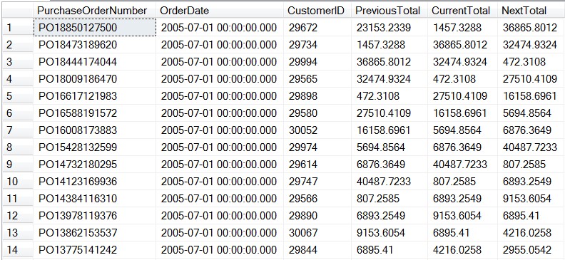
Recently I was tasked with calculating the difference between two values, however the values existed in different rows. My first thought was a self-join on the table and compare the two results. Using Adventure Works 2012, I ran the following query and the results are shown.

SELECT   soh.PurchaseOrderNumber
       , soh.OrderDate
       , soh.CustomerID
       , PreviousTotal = soh1.TotalDue
       , CurrentTotal = soh.TotalDue
       , NextTotal = soh2.TotalDue
FROM     Sales.SalesOrderHeader soh
JOIN     Sales.SalesOrderHeader soh1 ON soh1.SalesOrderID = soh.SalesOrderID - 1
JOIN     Sales.SalesOrderHeader soh2 ON soh2.SalesOrderID = soh.SalesOrderID + 1;

LagLeadImg1

This result set shows the previous and next record values for the TotalDue column. This got me 1/2 way to what was needed to perform the difference calculations. I needed the results for a given customer rather than all customers. I updated the query to allow for a customer ID to be passed into the query and the results are shown.

DECLARE @CustomerID int = 30117;
SELECT   soh.PurchaseOrderNumber
       , soh.OrderDate
       , soh.CustomerID
       , PreviousTotal = soh1.TotalDue
       , CurrentTotal = soh.TotalDue
       , NextTotal = soh2.TotalDue
FROM     Sales.SalesOrderHeader soh
LEFT JOIN Sales.SalesOrderHeader soh1 ON soh1.SalesOrderID = soh.SalesOrderID - 1
                                         AND soh1.CustomerID = soh.CustomerID
LEFT JOIN Sales.SalesOrderHeader soh2 ON soh2.SalesOrderID = soh.SalesOrderID + 1
                                         AND soh2.CustomerID = soh.CustomerID
WHERE    soh.CustomerID = @CustomerID;

LagLeadImg2

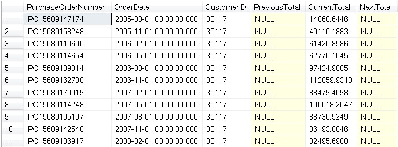
This is was a problem. Being that I was using the SalesOrderID to perform the self-joins on the tables, and the Customer’s records were not in sequential order, I was not getting any of the previous and next records.

LEAD()/LAG() OVER (PARTITION BY)

Instead of going down the path of craziness, I decided to eliminate the use of the self-referencing joins and opted to use the OVER clause with LEAD and LAG to solve the problem. Using the following query and output we can explain the LEAD(), LAG(), OVER (PARTITION BY) statements.

DECLARE @CustomerID int = 30117;
SELECT   PurchaseOrderNumber
       , OrderDate
       , CustomerID
       , CurrentTotalDue = TotalDue
FROM     Sales.SalesOrderHeader soh
WHERE    soh.CustomerID = @CustomerID;

LagLeadImg3

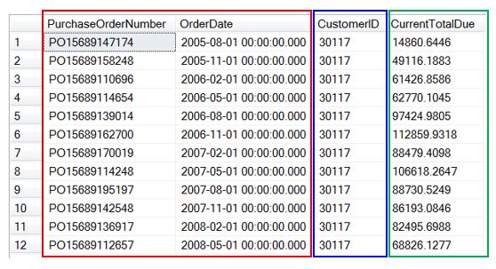
In the blue box is the CustomerID column, this is the column we want to Partition by.

In the red box is the PurchaseOrderNumber and OrderDate columns, these columns we want to order the results of the window.

In the green box is the CurrentTotalDue, this is the column that we will pass to the LEAD and LAG window functions.

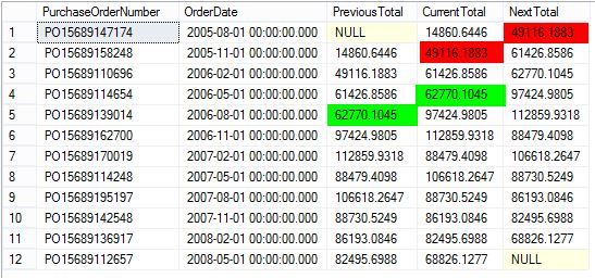
I updated the query to use the LEAD and LAG window functions and the results are shown. The red highlights show the results of the LEAD function and the green highlights show the results of the LAG function.

DECLARE @CustomerID int = 30117;
SELECT   PurchaseOrderNumber
       , OrderDate
       , PreviousTotal = LAG(TotalDue) OVER (PARTITION BY CustomerID ORDER BY OrderDate , PurchaseOrderNumber)
       , CurrentTotal = TotalDue
       , NextTotal = LEAD(TotalDue) OVER (PARTITION BY CustomerID ORDER BY OrderDate , PurchaseOrderNumber)
FROM     Sales.SalesOrderHeader soh
WHERE    soh.CustomerID = @CustomerID;

LagLeadImg5

As you can see the syntax for writing a query to use these LEAD and LAG are not overly complex. In a future blog post I will dive deeper into using the OVER statement.

Standard T-SQL UNPIVOT

In prior blog posts I talked about a Standard PIVOT query and a Dynamic PIVOT query. It is only fitting that I talk about how to implement an UNPIVOT query. As DBA’s we commonly unpivot data and turn it into normalized data for storing in a relational data store. Understanding how to use the UNPIVOT query is a great skill to have as a DBA. Just like the PIVOT operator, the UNPIVOT operator was introduced with SQL Server 2005. In this blog post I will show how we can use the UNPIVOT operator.

I got the idea for this blog post as a result from my online grade book. I noticed that the data is displayed as a denormalized set of data. As an instructor I thought it would be interesting to see average, sum, minimum and maximum assignment scores for each student. Below is an example of the display of the online grade book.

StudentID Assignment1 Assignment2 Assignment3 Assignment4
101 90 100 95 100
102 70 65 40 80
103 100 100 100 100

I found that writing a simple query to get the sum (adding each column) and average (adding each column and dividing by the number of columns) was not too bad. However, finding the minimum and maximum proved to be a bit tricky. Sure we could implement a CASE WHEN statement, however for each column the complexity and possibility of error increases significantly, and maintainability dang near goes out the window. In comes UNPIVOT to save the day. After unpivoting the data, we simply use the AVG(), SUM(), MIN() and MAX() functions.

Let’s take a look at the basic structure of the UNPIVOT query. Using the UNPIVOT statement, you specify a value and data column, then select each of the columns you want to unpivot into these new columns. The new value and data columns become select-able columns in the query, as shown in the following code.

SELECT   [AnyColumn]
       , [DataColumn]
       , [ValueColumn]
FROM     SomeTable ST 
UNPIVOT ( ValueColumn FOR DataColumn IN (UnPivotCol1, UnPivotCol2, UnPivotCol2) ) AS UNPVT

Applying this UNPIVOT syntax to our data above we yield the following query.

SELECT   StudentID
       , Assignment
       , ASMT.Score
FROM     #ClassGrades CG 
UNPIVOT ( Score FOR Assignment IN (Assignment1, Assignment2, Assignment3, Assignment4) ) AS ASMT

This query returns the following normalized view of the data

StudentID Assignment Score
101 Assignment1 90
101 Assignment2 100
101 Assignment3 95
101 Assignment4 100
102 Assignment1 70
102 Assignment2 65
102 Assignment3 40
102 Assignment4 80
103 Assignment1 100
103 Assignment2 100
103 Assignment3 100
103 Assignment4 100

Now that we have this data in a normalized result, applying SQL functions such as AVG() and SUM(), is relatively simple. Below is an updated version of the query using the AVG(), SUM(), MIN(), and MAX() functions grouping by StudentID.

SELECT   StudentID
       , Average = AVG(ASMT.Score)
	   , MaxScore = MAX(ASMT.Score)
	   , MinScore = MIN(ASMT.Score)
	   , Total = SUM(ASMT.Score)
FROM     #ClassGrades CG 
UNPIVOT ( Score FOR Assignment IN (Assignment1, Assignment2, Assignment3, Assignment4) ) AS ASMT
GROUP BY StudentID

This query returns the following view of the data

StudentID Average MaxScore MinScore Total
101 96 100 90 385
102 63 80 40 255
103 100 100 100 400

As you can see the PIVOT and UNPIVOT statements are not overly complex and are definitely great TSQL tools for any DBA to keep in their back-pocket. Below is the entire script with test data included.

IF OBJECT_ID('tempdb..#ClassGrades') IS NOT NULL 
   DROP TABLE #ClassGrades;
 
CREATE TABLE #ClassGrades (
   StudentID int PRIMARY KEY
                 NOT NULL
 , Assignment1 int NULL
 , Assignment2 int NULL
 , Assignment3 int NULL
 , Assignment4 int NULL);
 
INSERT   INTO #ClassGrades
         (StudentID, Assignment1, Assignment2, Assignment3, Assignment4)
VALUES   (101, 90, 100, 95, 100),
         (102, 70, 65, 40, 80),
         (103, 100, 100, 100, 100); 
 
SELECT   StudentID
       , Assignment
       , ASMT.Score
FROM     #ClassGrades CG 
UNPIVOT ( Score FOR Assignment IN (Assignment1, Assignment2, Assignment3, Assignment4) ) AS ASMT
 
SELECT   StudentID
       , Average = AVG(ASMT.Score)
	   , MaxScore = MAX(ASMT.Score)
	   , MinScore = MIN(ASMT.Score)
	   , Total = SUM(ASMT.Score)
FROM     #ClassGrades CG 
UNPIVOT ( Score FOR Assignment IN (Assignment1, Assignment2, Assignment3, Assignment4) ) AS ASMT
GROUP BY StudentID;